Applying digital filters in Python

Digital filters are an important tool in signal processing. The SciPy library provides functionality to design and apply different kinds of filters. It is designed for offline use and thus, however, not really suited for real-time applications. In the next post, I am highlighting how live versions of the SciPy filters are implemented in yarppg, a video-based heart rate measurement system. Before looking into the implementations, let’s discuss what digital filters can do and why they are so important in signal processing.

This post covers the following topics:

• an example application of a digital low-pass filter
• a brief description of infinite impulse response (IIR) filters
• designing IIR filters in scipy.signal
• applying the filter with lfilter and filtfilt

Digital filter applications

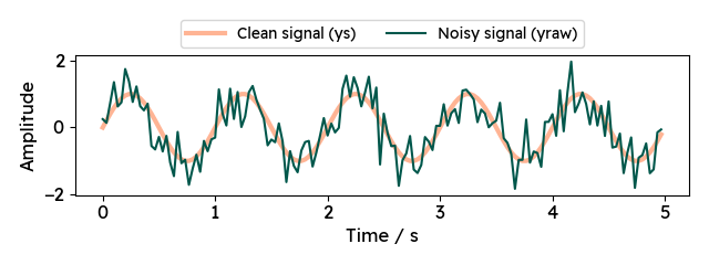
If you are measuring any signal in the real world, chances are that there is some degree of noise. Depending on the signal-to-noise ratio (SNR) and the application, this may or may not be a problem. In my previous post, for example, I am extracting a pulse signal from the average skin color of a person’s face. While the heartbeats are visible in the signal, there is a lot of flickering that impairs the detectability of pulse waves:

Here is where digital filters can help. We want to get rid of the high-frequency noise and extract the underlying signal of lower frequency. This can be achieved with a low-pass filter. As the name suggests, a low-pass filter rejects higher frequencies, while lower frequencies are not affected (“passed”). Other types are high-pass, band-pass and band-stop. Generally speaking, digital filters allow you to reduce or amplify the influence of certain frequency ranges in the signal.

Infinite impulse response (IIR) filters

There are different ways to define and use a digital filter in Python. The most versatile approach is using infinite impulse response (IIR) filters. An IIR filter is described by a so-called difference equation, which defines how an incoming signal is processed over time. A new output $y[n]$ is obtained by mathematically combining past filter outputs with past inputs (recursion)¹.

A difference equation looks something like this: $$ a_0 y[n] = b_0 x[n] + b_1 x[n-1] + b_2 x[n-2] - a_1 y[n-1] - a_2 y[n-2] $$ The new output is a weighted sum of past inputs and outputs. Depending on the actual values of the coefficients $a_i$ and $b_i$, such a filter can reject or pass certain frequency ranges. Higher order filters look further into the past and thus feature more terms than illustrated above. Finding suitable coefficients to achieve a desired behavior - a process called filter design - is a rich topic in itself. Luckily, we can leverage existing tools allowing users to not worry about this too much.

Filter design hyper-parameters

To use an IIR filter in Python, we first need to “design” it. There are several functions that do this. Here, I am using the iirfilter function provided in scipy.signal. The most important thing to decide is which frequency ranges we want to keep/reject. For the example signal above, we want to use a low-pass filter rejecting the rapid fluctuations of the noise. In other applications, we might want to only keep higher frequencies (high-pass) or limit the signal to a certain frequency range (band-pass).

Besides the filter type, we need to specify the critical frequency, above which the signal is attenuated. The synthetic example signal from before has a frequency of 1 Hz, but the critical frequency should be higher. Why? First, a digital filter is not perfect and it will dampen signals close to the critical frequency as well. Second (and more importantly), signals may not be limited exactly to the desired frequency range. Assuming the signal above represents a person’s pulse - the heart may well beat at a rate higher than 60 beats/min. In fact, we want to include a wider range of physiologically reasonable heart rates, up to 150 beats/min or 2.5 Hz.

There is one more required parameter for scipy.signal.iirfilter. The filter order dictates the number of terms in the difference equation. The order defines the sharpness of the frequency cutoff. The higher the order, the better the behavior close the the critical frequency. While this is generally desired, higher orders come at the cost of increased processing efforts and a signal delay (phase shift).

Finally, there are five different types of IIR filter designs you can choose from in iirfilter. There are several pros and cons to each design approach, which I am not competent enough to dive into. I tend to use the most common design, introduced by Butterworth² and have not yet needed to switch things up.

Designing and applying an IIR low-pass in Python

Let’s create a synthetic example, to which we can apply the filter. I am choosing a sampling rate of 30 Hz (typical FPS of a consumer webcam) and generate 5 seconds of a sine wave overlaid with Gaussian noise. yraw and ys are the signals plotted earlier.

1
2
3
4
5
6
7
8
9

import numpy as np
import scipy.signal

np.random.seed(42)  # for reproducibility
fs = 30  # sampling rate, Hz
ts = np.arange(0, 5, 1.0 / fs)  # time vector - 5 seconds
ys = np.sin(2*np.pi * 1.0 * ts)  # signal @ 1.0 Hz, without noise
yerr = 0.5 * np.random.normal(size=len(ts))  # Gaussian noise
yraw = ys + yerr

Now we can design the low-pass filter to cut off frequencies greater than 2.5 Hz. By default, the iirfilter function returns the coefficients of the difference equation $b_i$ and $a_i$, which can be passed to a filter function. The next post will deal with a different output format. I am choosing a filter order of 4 (first argument). The Butterworth filter type is the default choice, but it is better to be explicit. We can apply the designed filter on the noisy signal by calling the lfilter function.

1
2
3

b, a = scipy.signal.iirfilter(4, Wn=2.5, fs=fs, btype="low", ftype="butter")
print(b, a, sep="\n")
y_lfilter = scipy.signal.lfilter(b, a, yraw)

[0.003 0.01  0.015 0.01  0.003]
[1. -2.639  2.769 -1.339  0.25]

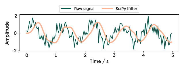
Let’s plot the raw and the low-pass-filtered signal:

 1
 2
 3
 4
 5
 6
 7
 8
 9
10
11

from matplotlib import pyplot as plt

plt.figure(figsize=[6.4, 2.4])

plt.plot(ts, yraw, label="Raw signal")
plt.plot(ts, y_lfilter, alpha=0.8, lw=3, label="SciPy lfilter")

plt.xlabel("Time / s")
plt.ylabel("Amplitude")
plt.legend(loc="lower center", bbox_to_anchor=[0.5, 1],
           ncol=2, fontsize="smaller")

Here, we can note two things. First, the initial signal is not properly recovered. A more narrow filter design could help, but as discussed above, that may not always be an option. Second, the signal is shifted slightly. This is because of the delay caused by the filter (phase shift).

Using filtfilt to achieve zero-phase filtering

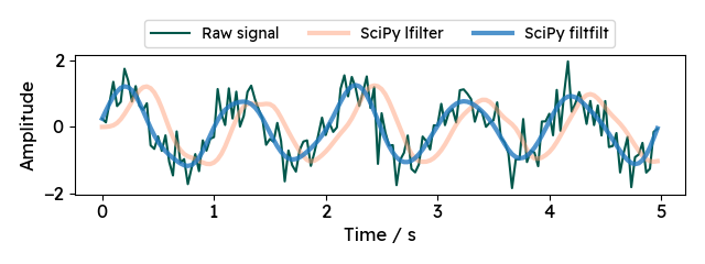
Phase shift is an inherent issue with digital filters and can only be properly dealt with, in an offline setting: if the entire signal is available, we can apply the filter twice - once forward, once backward. This way, the phase shift is compensated by the second run and the output signal is “in phase” with the input. The scipy.signal.filtfilt does exactly that. It can be used in the same way as lfilter:

1
2

# apply filter forward and backward using filtfilt
y_filtfilt = scipy.signal.filtfilt(b, a, yraw)

The resulting output is nicely aligned with the raw signal and even smoother compared to lfilter output. This is because by applying the filter twice, we are essentially doubling the order of the filter. Keep this in mind when designing the filter, you may be able to reduce the order beforehand, if you are only going to use filtfilt.

Both lfilter and filtfilt are easy to use and work well in an offline setting. But the scipy.signal functions are not designed for real-time applications. In the next post, I will show how to implement an IIR filter for live applications in just a few lines of code.

Btw, here is the complete code for this post:

 1
 2
 3
 4
 5
 6
 7
 8
 9
10
11
12
13
14
15
16
17
18
19
20
21
22
23
24
25
26
27
28
29
30
31
32
33
34
35
36
37
38
39
40
41
42
43
44
45
46
47
48
49
50
51
52
53
54
55
56
57

import numpy as np

from matplotlib import pyplot as plt
import scipy.signal

np.random.seed(42)  # for reproducibility
# create time steps and corresponding sine wave with Gaussian noise
fs = 30  # sampling rate, Hz
ts = np.arange(0, 5, 1.0 / fs)  # time vector - 5 seconds

ys = np.sin(2*np.pi * 1.0 * ts)  # signal @ 1.0 Hz, without noise
yerr = 0.5 * np.random.normal(size=len(ts))  # Gaussian noise
yraw = ys + yerr

# plot raw signal
plt.figure(figsize=[6.4, 2.4])
plt.plot(ts, ys, alpha=0.8, lw=3, color="C1", label="Clean signal (ys)")
plt.plot(ts, yraw, color="C0", label="Noisy signal (yraw)")
plt.xlabel("Time / s")
plt.ylabel("Amplitude")
plt.legend(loc="lower center", bbox_to_anchor=[0.5, 1], ncol=2,
           fontsize="smaller")

plt.tight_layout()
# plt.savefig("noisy-signal.png", dpi=100)

# define lowpass filter with 2.5 Hz cutoff frequency
b, a = scipy.signal.iirfilter(4, Wn=2.5, fs=fs, btype="low", ftype="butter")
print(b, a, sep="\n")
y_lfilter = scipy.signal.lfilter(b, a, yraw)

plt.figure(figsize=[6.4, 2.4])
plt.plot(ts, yraw, label="Raw signal")
plt.plot(ts, y_lfilter, alpha=0.8, lw=3, label="SciPy lfilter")
plt.xlabel("Time / s")
plt.ylabel("Amplitude")
plt.legend(loc="lower center", bbox_to_anchor=[0.5, 1], ncol=2,
           fontsize="smaller")

plt.tight_layout()
# plt.savefig("simple-lowpass-lfilter.png", dpi=100)

# apply filter forward and backward using filtfilt
y_filtfilt = scipy.signal.filtfilt(b, a, yraw)

plt.figure(figsize=[6.4, 2.4])
plt.plot(ts, yraw, label="Raw signal")
plt.plot(ts, y_lfilter, alpha=0.5, lw=3, label="SciPy lfilter")
plt.plot(ts, y_filtfilt, alpha=0.8, lw=3, label="SciPy filtfilt")
plt.legend(loc="lower center", bbox_to_anchor=[0.5, 1], ncol=3,
           fontsize="smaller")
plt.xlabel("Time / s")
plt.ylabel("Amplitude")

plt.tight_layout()
# plt.savefig("lowpass-filtfilt.png", dpi=100)
plt.show()

(References)